
Local to remote
Local to remote#
When developers write code they typically begin with a simple serial code and build upon it until all of the required functionality is present. The following set of examples were developed to demonstrate this iterative process of evolving a simple serial program to an efficient, fully-distributed HPX application. For this demonstration, we implemented a 1D heat distribution problem. This calculation simulates the diffusion of heat across a ring from an initialized state to some user-defined point in the future. It does this by breaking each portion of the ring into discrete segments and using the current segment’s temperature and the temperature of the surrounding segments to calculate the temperature of the current segment in the next timestep as shown by Fig. 2 below.
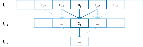
Fig. 2 Heat diffusion example program flow.#
We parallelize this code over the following eight examples:
The first example is straight serial code. In this code we instantiate a vector
U that contains two vectors of doubles as seen in the structure
stepper.
struct stepper
{
    // Our partition type
    typedef double partition;

    // Our data for one time step
    typedef std::vector<partition> space;

    // Our operator
    static double heat(double left, double middle, double right)
    {
        return middle + (k * dt / (dx * dx)) * (left - 2 * middle + right);
    }

    // do all the work on 'nx' data points for 'nt' time steps
    space do_work(std::size_t nx, std::size_t nt)
    {
        // U[t][i] is the state of position i at time t.
        std::vector<space> U(2);
        for (space& s : U)
            s.resize(nx);

        // Initial conditions: f(0, i) = i
        for (std::size_t i = 0; i != nx; ++i)
            U[0][i] = double(i);

        // Actual time step loop
        for (std::size_t t = 0; t != nt; ++t)
        {
            space const& current = U[t % 2];
            space& next = U[(t + 1) % 2];

            next[0] = heat(current[nx - 1], current[0], current[1]);

            for (std::size_t i = 1; i != nx - 1; ++i)
                next[i] = heat(current[i - 1], current[i], current[i + 1]);

            next[nx - 1] = heat(current[nx - 2], current[nx - 1], current[0]);
        }

        // Return the solution at time-step 'nt'.
        return U[nt % 2];
    }
};
Each element in the vector of doubles represents a single grid point. To
calculate the change in heat distribution, the temperature of each grid point,
along with its neighbors, is passed to the function heat. In order to
improve readability, references named current and next are created
which, depending on the time step, point to the first and second vector of
doubles. The first vector of doubles is initialized with a simple heat ramp.
After calling the heat function with the data in the current vector, the
results are placed into the next vector.
In example 2 we employ a technique called futurization. Futurization is a method
by which we can easily transform a code that is serially executed into a code
that creates asynchronous threads. In the simplest case this involves replacing
a variable with a future to a variable, a function with a future to a function,
and adding a .get() at the point where a value is actually needed. The code
below shows how this technique was applied to the struct stepper.
struct stepper
{
    // Our partition type
    typedef hpx::shared_future<double> partition;

    // Our data for one time step
    typedef std::vector<partition> space;

    // Our operator
    static double heat(double left, double middle, double right)
    {
        return middle + (k * dt / (dx * dx)) * (left - 2 * middle + right);
    }

    // do all the work on 'nx' data points for 'nt' time steps
    hpx::future<space> do_work(std::size_t nx, std::size_t nt)
    {
        using hpx::dataflow;
        using hpx::unwrapping;

        // U[t][i] is the state of position i at time t.
        std::vector<space> U(2);
        for (space& s : U)
            s.resize(nx);

        // Initial conditions: f(0, i) = i
        for (std::size_t i = 0; i != nx; ++i)
            U[0][i] = hpx::make_ready_future(double(i));

        auto Op = unwrapping(&stepper::heat);

        // Actual time step loop
        for (std::size_t t = 0; t != nt; ++t)
        {
            space const& current = U[t % 2];
            space& next = U[(t + 1) % 2];

            // WHEN U[t][i-1], U[t][i], and U[t][i+1] have been computed, THEN we
            // can compute U[t+1][i]
            for (std::size_t i = 0; i != nx; ++i)
            {
                next[i] =
                    dataflow(hpx::launch::async, Op, current[idx(i, -1, nx)],
                        current[i], current[idx(i, +1, nx)]);
            }
        }

        // Now the asynchronous computation is running; the above for-loop does not
        // wait on anything. There is no implicit waiting at the end of each timestep;
        // the computation of each U[t][i] will begin as soon as its dependencies
        // are ready and hardware is available.

        // Return the solution at time-step 'nt'.
        return hpx::when_all(U[nt % 2]);
    }
};
In example 2, we redefine our partition type as a shared_future and, in
main, create the object result, which is a future to a vector of
partitions. We use result to represent the last vector in a string of
vectors created for each timestep. In order to move to the next timestep, the
values of a partition and its neighbors must be passed to heat once the
futures that contain them are ready. In HPX, we have an LCO (Local Control
Object) named Dataflow that assists the programmer in expressing this
dependency. Dataflow allows us to pass the results of a set of futures to a
specified function when the futures are ready. Dataflow takes three types of
arguments, one which instructs the dataflow on how to perform the function call
(async or sync), the function to call (in this case Op), and futures to the
arguments that will be passed to the function. When called, dataflow immediately
returns a future to the result of the specified function. This allows users to
string dataflows together and construct an execution tree.
After the values of the futures in dataflow are ready, the values must be pulled
out of the future container to be passed to the function heat. In order to
do this, we use the HPX facility unwrapping, which underneath calls
.get() on each of the futures so that the function heat will be passed
doubles and not futures to doubles.
By setting up the algorithm this way, the program will be able to execute as quickly as the dependencies of each future are met. Unfortunately, this example runs terribly slow. This increase in execution time is caused by the overheads needed to create a future for each data point. Because the work done within each call to heat is very small, the overhead of creating and scheduling each of the three futures is greater than that of the actual useful work! In order to amortize the overheads of our synchronization techniques, we need to be able to control the amount of work that will be done with each future. We call this amount of work per overhead grain size.
In example 3, we return to our serial code to figure out how to control the
grain size of our program. The strategy that we employ is to create “partitions”
of data points. The user can define how many partitions are created and how many
data points are contained in each partition. This is accomplished by creating
the struct partition, which contains a member object data_, a vector of
doubles that holds the data points assigned to a particular instance of
partition.
In example 4, we take advantage of the partition setup by redefining space
to be a vector of shared_futures with each future representing a partition. In
this manner, each future represents several data points. Because the user can
define how many data points are in each partition, and, therefore, how
many data points are represented by one future, a user can control the
grainsize of the simulation. The rest of the code is then futurized in the same
manner as example 2. It should be noted how strikingly similar
example 4 is to example 2.
Example 4 finally shows good results. This code scales equivalently to the OpenMP version. While these results are promising, there are more opportunities to improve the application’s scalability. Currently, this code only runs on one locality, but to get the full benefit of HPX, we need to be able to distribute the work to other machines in a cluster. We begin to add this functionality in example 5.
In order to run on a distributed system, a large amount of boilerplate code must
be added. Fortunately, HPX provides us with the concept of a component,
which saves us from having to write quite as much code. A component is an object
that can be remotely accessed using its global address. Components are made of
two parts: a server and a client class. While the client class is not required,
abstracting the server behind a client allows us to ensure type safety instead
of having to pass around pointers to global objects. Example 5 renames example
4’s struct partition to partition_data and adds serialization support.
Next, we add the server side representation of the data in the structure
partition_server. Partition_server inherits from
hpx::components::component_base, which contains a server-side component
boilerplate. The boilerplate code allows a component’s public members to be
accessible anywhere on the machine via its Global Identifier (GID). To
encapsulate the component, we create a client side helper class. This object
allows us to create new instances of our component and access its members
without having to know its GID. In addition, we are using the client class to
assist us with managing our asynchrony. For example, our client class
partition‘s member function get_data() returns a future to
partition_data get_data(). This struct inherits its boilerplate code from
hpx::components::client_base.
In the structure stepper, we have also had to make some changes to
accommodate a distributed environment. In order to get the data from a
particular neighboring partition, which could be remote, we must retrieve the data from all
of the neighboring partitions. These retrievals are asynchronous and the function
heat_part_data, which, amongst other things, calls heat, should not be
called unless the data from the neighboring partitions have arrived. Therefore,
it should come as no surprise that we synchronize this operation with another
instance of dataflow (found in heat_part). This dataflow receives futures
to the data in the current and surrounding partitions by calling get_data()
on each respective partition. When these futures are ready, dataflow passes them
to the unwrapping function, which extracts the shared_array of doubles and
passes them to the lambda. The lambda calls heat_part_data on the
locality, which the middle partition is on.
Although this example could run distributed, it only runs on one
locality, as it always uses hpx::find_here() as the target for the
functions to run on.
In example 6, we begin to distribute the partition data on different nodes. This
is accomplished in stepper::do_work() by passing the GID of the
locality where we wish to create the partition to the partition
constructor.
    for (std::size_t i = 0; i != np; ++i)
        U[0][i] = partition(localities[locidx(i, np, nl)], nx, double(i));
We distribute the partitions evenly based on the number of localities used,
which is described in the function locidx. Because some of the data needed
to update the partition in heat_part could now be on a new locality,
we must devise a way of moving data to the locality of the middle
partition. We accomplished this by adding a switch in the function
get_data() that returns the end element of the buffer data_ if it is
from the left partition or the first element of the buffer if the data is from
the right partition. In this way only the necessary elements, not the whole
buffer, are exchanged between nodes. The reader should be reminded that this
exchange of end elements occurs in the function get_data() and, therefore, is
executed asynchronously.
Now that we have the code running in distributed, it is time to make some
optimizations. The function heat_part spends most of its time on two tasks:
retrieving remote data and working on the data in the middle partition. Because
we know that the data for the middle partition is local, we can overlap the work
on the middle partition with that of the possibly remote call of get_data().
This algorithmic change, which was implemented in example 7, can be seen below:
    // The partitioned operator, it invokes the heat operator above on all elements
    // of a partition.
    static partition heat_part(
        partition const& left, partition const& middle, partition const& right)
    {
        using hpx::dataflow;
        using hpx::unwrapping;

        hpx::shared_future<partition_data> middle_data =
            middle.get_data(partition_server::middle_partition);

        hpx::future<partition_data> next_middle = middle_data.then(
            unwrapping([middle](partition_data const& m) -> partition_data {
                HPX_UNUSED(middle);

                // All local operations are performed once the middle data of
                // the previous time step becomes available.
                std::size_t size = m.size();
                partition_data next(size);
                for (std::size_t i = 1; i != size - 1; ++i)
                    next[i] = heat(m[i - 1], m[i], m[i + 1]);
                return next;
            }));

        return dataflow(hpx::launch::async,
            unwrapping([left, middle, right](partition_data next,
                           partition_data const& l, partition_data const& m,
                           partition_data const& r) -> partition {
                HPX_UNUSED(left);
                HPX_UNUSED(right);

                // Calculate the missing boundary elements once the
                // corresponding data has become available.
                std::size_t size = m.size();
                next[0] = heat(l[size - 1], m[0], m[1]);
                next[size - 1] = heat(m[size - 2], m[size - 1], r[0]);

                // The new partition_data will be allocated on the same locality
                // as 'middle'.
                return partition(middle.get_id(), std::move(next));
            }),
            std::move(next_middle),
            left.get_data(partition_server::left_partition), middle_data,
            right.get_data(partition_server::right_partition));
    }
Example 8 completes the futurization process and utilizes the full potential of
HPX by distributing the program flow to multiple localities, usually defined as
nodes in a cluster. It accomplishes this task by running an instance of HPX main
on each locality. In order to coordinate the execution of the program,
the struct stepper is wrapped into a component. In this way, each
locality contains an instance of stepper that executes its own instance
of the function do_work(). This scheme does create an interesting
synchronization problem that must be solved. When the program flow was being
coordinated on the head node, the GID of each component was known. However, when
we distribute the program flow, each partition has no notion of the GID of its
neighbor if the next partition is on another locality. In order to make
the GIDs of neighboring partitions visible to each other, we created two buffers
to store the GIDs of the remote neighboring partitions on the left and right
respectively. These buffers are filled by sending the GID of newly created
edge partitions to the right and left buffers of the neighboring localities.
In order to finish the simulation, the solution vectors named result are then
gathered together on locality 0 and added into a vector of spaces
overall_result using the HPX functions gather_id and gather_here.
Example 8 completes this example series, which takes the serial code of example 1 and incrementally morphs it into a fully distributed parallel code. This evolution was guided by the simple principles of futurization, the knowledge of grainsize, and utilization of components. Applying these techniques easily facilitates the scalable parallelization of most applications.